Machine Learning Course

Trener
Krzysztof Mędrela
tel.: +48 660 873 898
email: krzysztof@medrela.com
web: www.medrela.com

Installation

Create universe.py File

Create universe.py file and put the following code there:

# %%writefile universe.py
# Ignore warning
import warnings
warnings.filterwarnings('ignore', message="numpy.dtype size changed")
warnings.filterwarnings('ignore', message="Objective did not converge")
warnings.filterwarnings('ignore', message=r"The \*bottom\* kwarg to \`barh\` is deprecated use \*y\* instead\.")
warnings.filterwarnings('ignore', message=r".*Falling back to \'gelss\' driver")
warnings.filterwarnings('ignore', message=r"Variables are collinear")
warnings.filterwarnings('ignore', message="Precision is ill-defined")
warnings.filterwarnings('ignore', message="invalid value encountered in double_scalars")
warnings.filterwarnings('ignore', message="F-score is ill-defined")
warnings.filterwarnings('ignore', message="Precision and F-score are ill-defined")
warnings.filterwarnings('ignore', message="The 'categorical_features' keyword is deprecated in version")
warnings.filterwarnings('ignore', message="posx and posy should be finite values")
# warnings.filterwarnings('ignore', category=DeprecationWarning)
# warnings.filterwarnings('ignore', category=FutureWarning)
# warnings.filterwarnings("ignore", message="numpy.core.umath_tests is an internal NumPy module")

# Builtin Libraries
from collections import defaultdict
from datetime import date
from datetime import datetime
from itertools import chain, combinations
from optparse import OptionParser
import pickle
import sys

# Third-party backports of builtin libraries
# from dataclasses import dataclass

# Third-party Libraries
# import graphviz
import matplotlib as mpl
from matplotlib import pyplot as plt
import mglearn
import numpy as np
import pandas as pd
from scipy.cluster.hierarchy import dendrogram, ward
import scipy.linalg

# Ignore some warnings from numpy
np.seterr(divide='ignore', invalid='ignore')

# Datasets Builtin Into scikit-learn
from mglearn.datasets import make_blobs as mglearn_make_blobs
from sklearn.datasets import load_boston
from sklearn.datasets import load_breast_cancer
from sklearn.datasets import load_digits
from sklearn.datasets import load_iris
from sklearn.datasets import make_blobs
from sklearn.datasets import make_moons

# Utilities from scikit-learn
from sklearn.cross_decomposition import PLSRegression
from sklearn.decomposition import PCA
from sklearn.decomposition import NMF
from sklearn.feature_selection import RFE
from sklearn.feature_selection import SelectFromModel
from sklearn.feature_selection import SelectPercentile
from sklearn.feature_selection import SelectKBest
from sklearn.manifold import TSNE
from sklearn.model_selection import cross_val_score
from sklearn.model_selection import GridSearchCV
from sklearn.model_selection import GroupKFold
from sklearn.model_selection import KFold
from sklearn.model_selection import LeaveOneOut
from sklearn.model_selection import PredefinedSplit
from sklearn.model_selection import ShuffleSplit
from sklearn.model_selection import StratifiedKFold
from sklearn.model_selection import StratifiedShuffleSplit
from sklearn.model_selection import TimeSeriesSplit
from sklearn.model_selection import train_test_split
from sklearn.pipeline import Pipeline
from sklearn.preprocessing import MinMaxScaler
from sklearn.preprocessing import OneHotEncoder
from sklearn.preprocessing import PolynomialFeatures
from sklearn.preprocessing import StandardScaler
from sklearn.preprocessing import FunctionTransformer

# Metrics
from sklearn.metrics import accuracy_score
from sklearn.metrics import average_precision_score
from sklearn.metrics import classification_report
from sklearn.metrics import cohen_kappa_score
from sklearn.metrics import confusion_matrix
from sklearn.metrics import f1_score
from sklearn.metrics import fbeta_score
from sklearn.metrics import make_scorer
from sklearn.metrics import precision_recall_curve
from sklearn.metrics import roc_auc_score
from sklearn.metrics import roc_curve
from sklearn.metrics.cluster import adjusted_rand_score

# Models from scikit-learn
from sklearn.cluster import AgglomerativeClustering
from sklearn.cluster import DBSCAN
from sklearn.cluster import KMeans
from sklearn.discriminant_analysis import LinearDiscriminantAnalysis
from sklearn.discriminant_analysis import QuadraticDiscriminantAnalysis
from sklearn.dummy import DummyClassifier
from sklearn.ensemble import BaggingRegressor
from sklearn.ensemble import GradientBoostingClassifier
from sklearn.ensemble import GradientBoostingRegressor
from sklearn.ensemble import RandomForestClassifier
from sklearn.ensemble import RandomForestRegressor
from sklearn.linear_model import ElasticNet
from sklearn.linear_model import Lasso
from sklearn.linear_model import LinearRegression
from sklearn.linear_model import LogisticRegression
from sklearn.linear_model import Ridge
from sklearn.naive_bayes import GaussianNB
from sklearn.naive_bayes import MultinomialNB
from sklearn.neighbors import KNeighborsClassifier
from sklearn.neighbors import KNeighborsRegressor
from sklearn.neural_network import MLPClassifier
from sklearn.svm import SVC
from sklearn.tree import DecisionTreeClassifier
from sklearn.tree import DecisionTreeRegressor
from sklearn.tree import export_graphviz

# imbalanced-learn
#from imblearn.under_sampling import RandomUnderSampler
#from imblearn.over_sampling import RandomOverSampler

# Deep Learning
# import keras
# from keras.datasets import boston_housing
# from keras.datasets import cifar10
# from keras.datasets import mnist
# from keras.layers import Conv2D
# from keras.layers import Dense
# from keras.layers import Dropout
# from keras.layers import Flatten
# from keras.layers import LSTM
# from keras.layers import MaxPooling2D
# from keras.models import load_model
# from keras.models import Sequential
# from keras.preprocessing.image import ImageDataGenerator
# from keras.utils import to_categorical
# import tensorflow

# Finish
python_version = sys.version.split(" ")[0]
print(f"Python version: {python_version}")
print("Universe has been successfully imported.")

from universe import *

Data Visualization with matplotlib

%matplotlib inline

from matplotlib import pyplot as plt

Basic Line Plots

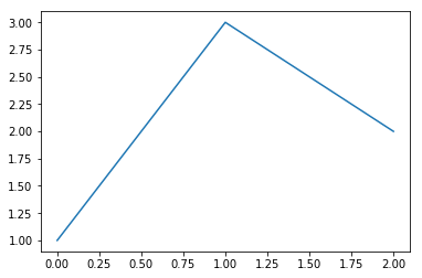
Y

plt.figure(figsize=(10, 5))
plt.plot([1, 3, 2])
plt.show()

[<matplotlib.lines.Line2D at 0x10c17c668>]

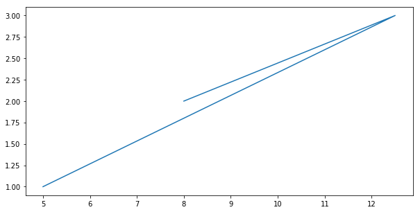
X and Y

plt.figure(figsize=(10, 5))
x = [5.0, 12.5, 8.0]
y = [1, 3, 2]
plt.plot(x, y)
plt.show()

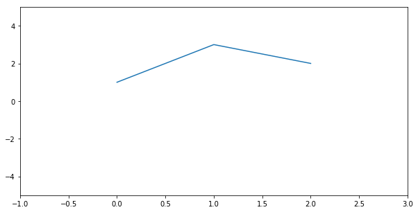
Custom Area

plt.figure(figsize=(10, 5))
plt.plot([1, 3, 2])
plt.xlim(-1, 3)  # Setter
plt.ylim(-5, 5)
print(plt.xlim())  # Getter
plt.show()

(-1.0, 3.0)

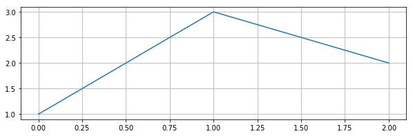
Grid

plt.figure(figsize=(10, 3))
plt.plot([1, 3, 2])
plt.grid()
plt.show()

Multiple Series

plt.figure(figsize=(10, 5))
plt.plot([1, 3, 2])  # First Series
plt.plot([5, 4, 1.5])  # Second Series
plt.show()

Legend

plt.figure(figsize=(10, 5))
plt.plot([1, 3, 2], label='A')
plt.plot([5, 4, 1.5])
plt.legend()  # loc='lower left'
plt.show()

Texts

plt.figure(figsize=(10, 5))
plt.plot([5.0, 5.5, 7.0], [1, 3, 2])
plt.title('Title')
plt.xlabel('xlabel')
plt.ylabel('ylabel')
plt.show()

Custom Line Style

plt.figure(figsize=(10, 5))
# Hit shift+Tab for more options
plt.plot([1, 3, 2], 'r--')  # r=red
plt.plot([5, 4, 1.5], 'gx')  # g=green
plt.show()
# Hit Shift+Tab for more customization options.

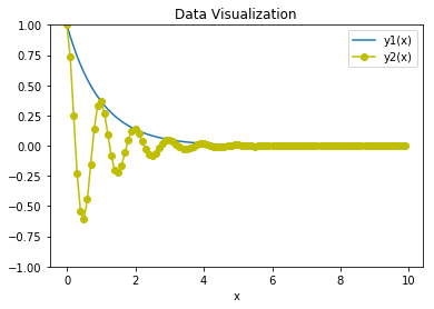
Exercise: Basic Line Plots

### Data

import numpy as np
from matplotlib import pyplot as plt

# Generating Data
x = np.arange(0.0, 10.0, 0.1)
y1 = np.exp(-x)
y2 = np.exp(-x) * np.cos(2*np.pi*x)

# Printing Data
print(f"x[:7] =  {x[:7]}")
print(f"y1[:4] = {y1[:4]}")
print(f"y2[:4] = {y2[:4]}")

x[:7] =  [0.  0.1 0.2 0.3 0.4 0.5 0.6]
y1[:4] = [1.         0.90483742 0.81873075 0.74081822]
y2[:4] = [ 1.          0.73202885  0.25300172 -0.22892542]

### Your Code Here
# y - yellow
# b - blue
# o - circle

### Solution
plt.figure()
plt.plot(x, y1, label="y1(x)")
plt.plot(x, y2, 'yo-', label="y2(x)")
plt.xlabel("x")
plt.ylim(-1, 1)
plt.legend()
plt.title("Data Visualization")
plt.show()

Scales

Linear Scale

plt.figure(figsize=(10, 5))
plt.plot([1, 100, 10, 5, 3, 1])
# plt.yscale('log')  # 'linear', log', 'symlog', 'logit'
plt.grid()
plt.show()

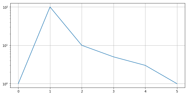
Log Scale

plt.figure(figsize=(10, 5))
plt.plot([1, 100, 10, 5, 3, 1])
plt.yscale('log')  # 'linear', log', 'symlog', 'logit'
plt.grid()
plt.show()

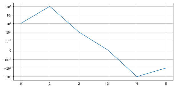
Symlog Scale

plt.figure(figsize=(10, 5))
plt.plot([10, 1000, 1, 0, -10, -1])
plt.yscale('symlog', linthreshy=0.1)
plt.grid()
plt.show()

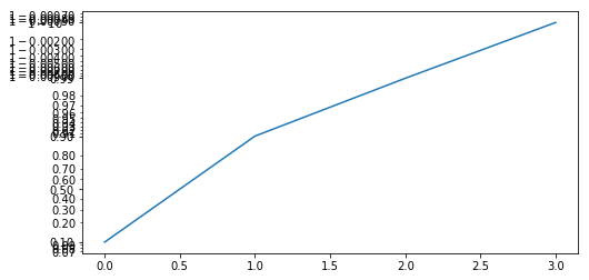
Logit Scale

plt.figure(figsize=(8, 4))
plt.plot([0.1, 0.9, 0.99, 0.999])
plt.yscale('logit')
plt.show()

Exercise: Scales

### Solution
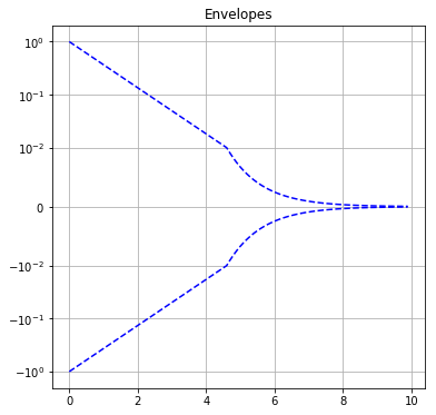
plt.figure(figsize=(6,6))
plt.yscale('symlog', linthreshy=0.01)
plt.plot(x, y1, 'b--')
plt.plot(x, -y1, 'b--')
plt.title("Envelopes")
plt.grid()

Multiple Plots

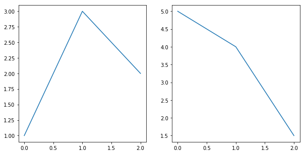
Subplot

plt.figure(figsize=(10, 5))

plt.subplot(1, 2, 1)
plt.plot([1, 3, 2])

plt.subplot(1, 2, 2)
plt.plot([5, 4, 1.5])

plt.show()

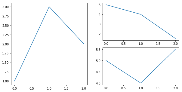
More Advanced Subplot

plt.figure(figsize=(10, 5))
plt.subplot(1, 2, 1)  # left half
plt.plot([1, 3, 2])  
plt.subplot(2, 2, 2)  # right top
plt.plot([5, 4, 1.5])  
plt.subplot(2, 2, 4)  # right bottom
plt.plot([5, 4, 5.5])
plt.show()

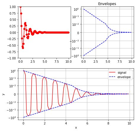
Exercise: Multiple Plots

### Data

import numpy as np
from matplotlib import pyplot as plt

# Generating Data
x = np.arange(0.0, 10.0, 0.1)
y1 = np.exp(-x)
y2 = np.exp(-x) * np.cos(2*np.pi*x)

# Printing Data
print(f"x[:7] =  {x[:7]}")
print(f"y1[:4] = {y1[:4]}")
print(f"y2[:4] = {y2[:4]}")

x[:7] =  [0.  0.1 0.2 0.3 0.4 0.5 0.6]
y1[:4] = [1.         0.90483742 0.81873075 0.74081822]
y2[:4] = [ 1.          0.73202885  0.25300172 -0.22892542]

# Your Code Here

### Solution

plt.figure(figsize=(7, 7))

plt.subplot(2, 2, 1)
plt.plot(x, y2, 'ro-')
plt.ylim(-1, 1)

plt.subplot(2, 2, 2)
plt.yscale('symlog', linthreshy=0.01)
plt.plot(x, y1, 'b--')
plt.plot(x, -y1, 'b--')
plt.title("Envelopes")
plt.grid()

plt.subplot(2, 1, 2)
plt.yscale('symlog', linthreshy=0.01)
plt.plot(x, y2, 'r', label="signal")
plt.plot(x, y1, 'b--', label="envelope")
plt.plot(x, -y1, 'b--')
plt.xlabel("x")
plt.ylabel("y")
plt.legend()
plt.grid()

plt.show()

Introduction to Machine Learning

from universe import *

Python version: 3.6.4
Universe has been successfully imported.

What is Machine Learning?

Artificial Intelligence -- intelligence demonstrated by machines, in contrast to the natural intelligence displayed by humans and other animals.

Machine Learning -- part of AI, a field of computer science that uses statistical techniques to give computer systems the ability to "learn" (e.g., progressively improve performance on a specific task) with data, without being explicitly programmed.

Deep Learning -- part of Machine Learning, part of a broader family of machine learning methods based on learning data representations, as opposed to task-specific algorithms. To cut the long story short, it's all about neural networks.

Basic Concepts

Petal vs sepal

Input: petal and sepal lengths and widths.

Multiclass output: setosa, versicolor, or virginica.

Data

Basic Concepts

• Dataset = a table of data
• Feature = one input column
• Featureset = all input columns
• Sample, data point, observation = one row
• Model or algorithm = a black box
• Input data, input, featureset, X = all input columns
• Output data, output, Y, target = the column that we want to predict
• Feature engineering and selection = choosing the best data representation
• Training and test data/set
• Supervised Learning = learning with the ground truth
• Unsupervised Learning = learning without ground truth
• Data type = either continuous (float or integer) or a category (binary or integer)

Case Study: Iris Classification

Step 1: Gather Data

Nothing to do. :-)

Step 2: Load Data

from universe import *
iris_dataset = load_iris()
X = iris_dataset['data']
y = iris_dataset['target']
np.random.seed(0)
y[::3] = np.random.randint(0, 3, size=(y.size//3))  # add some noise

print(X.shape)

(150, 4)

print(iris_dataset['feature_names'])

['sepal length (cm)', 'sepal width (cm)', 'petal length (cm)', 'petal width (cm)']

print(iris_dataset['target_names'])

['setosa' 'versicolor' 'virginica']

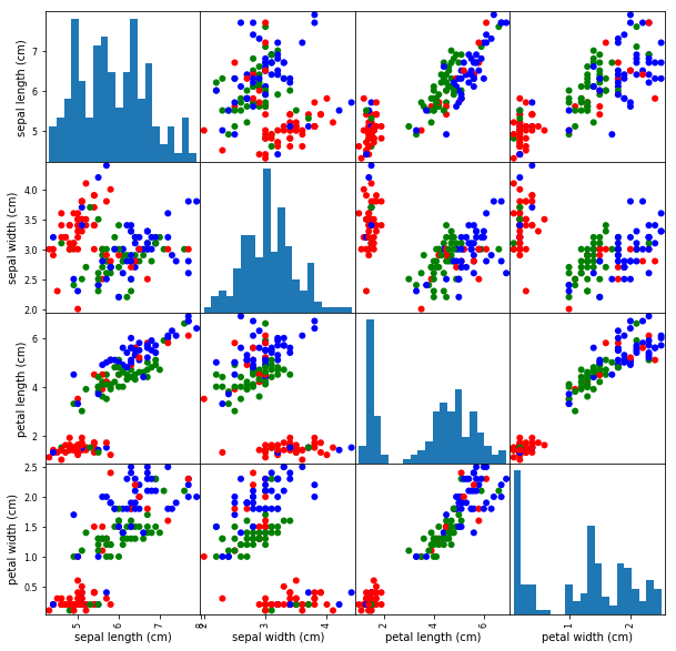
Step 3: Explore & Visualise Data

print(X[:5])

[[5.1 3.5 1.4 0.2]
 [4.9 3.  1.4 0.2]
 [4.7 3.2 1.3 0.2]
 [4.6 3.1 1.5 0.2]
 [5.  3.6 1.4 0.2]]

print(y)

[0 0 0 1 0 0 0 0 0 1 0 0 1 0 0 2 0 0 0 0 0 2 0 0 0 0 0 0 0 0 0 0 0 2 0 0 1
 0 0 2 0 0 2 0 0 0 0 0 1 0 1 1 1 1 1 1 1 1 1 1 0 1 1 1 1 1 0 1 1 0 1 1 1 1
 1 2 1 1 0 1 1 2 1 1 0 1 1 1 1 1 1 1 1 2 1 1 0 1 1 1 2 2 1 2 2 1 2 2 0 2 2
 2 2 2 0 2 2 2 2 2 2 2 2 0 2 2 2 2 2 0 2 2 0 2 2 0 2 2 1 2 2 1 2 2 2 2 2 0
 2 2]

X_df = pd.DataFrame(X, columns=iris_dataset['feature_names'])
X_df['category'] = y
display(X_df[:5])

	sepal length (cm)	sepal width (cm)	petal length (cm)	petal width (cm)	category
0	5.1	3.5	1.4	0.2	0
1	4.9	3.0	1.4	0.2	0
2	4.7	3.2	1.3	0.2	0
3	4.6	3.1	1.5	0.2	1
4	5.0	3.6	1.4	0.2	0

X_df = pd.DataFrame(X, columns=iris_dataset['feature_names'])
pd.plotting.scatter_matrix(
    X_df, 
    c=y,
    figsize=(10, 10),
    marker='o',
    hist_kwds={'bins': 20},
    alpha=1.0,
    cmap=mpl.colors.ListedColormap(['r', 'g', 'b']),
);

Step 4: Clean Data

Nothing to do. :-)

Step 5: Choose Data Representation

Let's stick to the original featureset.

Step 6: Build and Train Model

Step 6a: Train and Test Datasets

# Split dataset into train and test sets
X_train, X_test, y_train, y_test = train_test_split(
    X, y, random_state=0)

print(f"X_train.shape = {X_train.shape}")
print(f"X_test.shape  = {X_test.shape}")
print(f"y_train.shape = {y_train.shape}")
print(f"y_test.shape  = {y_test.shape}")

X_train.shape = (112, 4)
X_test.shape  = (38, 4)
y_train.shape = (112,)
y_test.shape  = (38,)

print(y_test)

[0 1 2 2 0 2 0 1 1 1 2 1 1 1 1 0 0 1 0 0 2 0 0 0 2 0 0 1 2 0 2 0 0 2 0 1 0
 1]

Step 6b: Build and Train Model

knn = KNeighborsClassifier(n_neighbors=1)  # Build Model
knn.fit(X_train, y_train);  # Train Model

Step 7: Evaluate Model

y_pred = knn.predict(X_test)
print(y_pred)

[2 1 0 2 2 2 0 1 1 1 2 1 1 1 1 0 1 1 0 0 2 1 0 0 0 0 0 1 1 0 2 1 0 1 2 1 0
 2]

print(np.mean(y_pred == y_test))
print(knn.score(X_test, y_test))  # Exactly the same as above

0.7105263157894737
0.7105263157894737

print(knn.score(X_train, y_train))

1.0

Complete Script

from universe import *

# Step 1: Gather Data
# nothing to do

# Step 2: Load Data
iris_dataset = load_iris()
X = iris_dataset['data']
y = iris_dataset['target']
np.random.seed(0)
y[::3] = np.random.randint(0, 3, size=(y.size//3))  # add some noise

# Step 3: Visualize and Explore Data
X_df = pd.DataFrame(X, columns=iris_dataset['feature_names'])
pd.plotting.scatter_matrix(
    X_df, 
    c=y,
    figsize=(10, 10),
    marker='o',
    hist_kwds={'bins': 20},
    alpha=1.0,
    cmap=mpl.colors.ListedColormap(['r', 'g', 'b']),
)

# Step 4: Clean Data
# nothing to do

# Step 5: Choose Data Representation
# Step 5a: Data Preprocessing (i.e. Normalization)
# Step 5b: Feature Engineering
# Step 5c: Feature Selection
# nothing to do

# Step 6: Build and Train Model
# Split dataset into train and test sets
X_train, X_test, y_train, y_test = train_test_split(
    X, y, random_state=0)

knn = KNeighborsClassifier(n_neighbors=1)  # Build Model
knn.fit(X_train, y_train)  # Train Model

# Step 7: Evaluate Model
prediction = knn.predict(np.array([[5, 2.9, 1 ,0.2]]))
train_score = knn.score(X_train, y_train)
test_score = knn.score(X_test, y_test)
print(f"TRAINING SCORE: {train_score:.3f}")
print(f"TEST SCORE: {test_score:.3f}")

TRAINING SCORE: 1.000
TEST SCORE: 0.711

Common Workflow

1. Gathering Data
2. Loading Data
3. Data Exploration and Visualization
4. Cleaning
5. Choosing Data Representation
   1. Data Preprocessing (i.e. Normalization)
   2. Feature Engineering
   3. Feature Selection
6. Building and Training a Model
7. Evaluating the Model

Problem Types

Algorithm cheat-sheet

Supervised Learning

Bias-Variance Trade Off

Underfitting and Overfitting

Bias and Variance

• The bias is an error from erroneous assumptions in the learning algorithm. High bias can cause an algorithm to miss the relevant relations between features and target outputs (underfitting).
• The variance is an error from sensitivity to small fluctuations in the training set. High variance can cause an algorithm to model the random noise in the training data, rather than the intended outputs (overfitting).

Sweet Spot

KNN Complexity

Iris Dataset

Resources

• Book: Introduction to Machine Learning with Python by Andreas C. Muller along with code snippets
• Scikit-learn Documentation (User Guide)
• Kaggle.com - data science projects

Regression Linear Models

from universe import *

Python version: 3.6.4
Universe has been successfully imported.

%matplotlib inline

Simple Linear Regression

Model & Cost Function

Model:

$$ y_\textit{prediction} = w \cdot x + b$$

Cost function (Ordinary Least Squares):

$$ \underset{w, b}{min\,} \frac{1}{2n_{samples}} \sum\limits_{i}^{\text{samples}} (y_\textit{prediction} - y_\textit{ground truth})^2 $$

Example Model

from universe import *

# Load and Split Data
X, y = mglearn.datasets.make_wave(n_samples=60)
y += 1.5
X_train, X_test, y_train, y_test = train_test_split(X, y, random_state=42)

# Build and Train Model
model = LinearRegression()
model.fit(X_train, y_train);

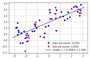
The Dataset

### Solution
# Evaluate Model
train_score = model.score(X_train, y_train)
test_score = model.score(X_test, y_test)

# Plot Figure
plt.figure()
plt.plot(X_train, y_train, 'bo', 
         label=f"train set (score: {train_score:.3f})")
plt.plot(X_test, y_test, 'ro', 
         label=f"test set (score: {test_score:.3f})")
# xx = np.linspace(*plt.xlim()).reshape(-1, 1)
xx = np.array(plt.xlim()).reshape(-1, 1)
yy = model.predict(xx)
plt.plot(xx, yy, 'k', 
         label=f"model: y = {model.coef_[0]:.3f}*x "
               f"+ {model.intercept_:.3f}")
plt.legend()
plt.grid()
plt.show()

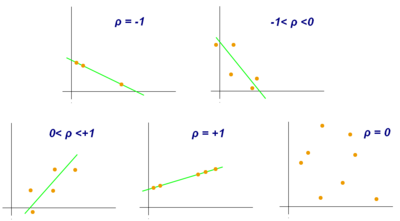
Correlation

correlation = np.corrcoef(X_train.reshape(-1), y_train)[0, 1]
print(f"CORRELATION:  {correlation:.3f}")
print(f"COEFFICIENTS: {model.coef_}")
print(f"INTERCEPT:    {model.intercept_}")

CORRELATION:  0.819
COEFFICIENTS: [0.39390555]
INTERCEPT:    1.4681956569732402

Multiple Linear Regression

Model & Cost Function

Model ($k$ features):

$$ y_\textit{prediction} = w_1 \cdot x_1 + \dots + w_k \cdot x_k + b$$

Cost function (Ordinary Least Squares):

$$ \underset{w_1,\dots,w_k,b}{min\,} \frac{1}{2n_{samples}} \sum\limits_{i}^{\text{samples}} (y_\textit{prediction} - y_\textit{ground truth})^2 $$

Boston Dataset

Boston dataset has 13 features.

The output is median value of owner-occupied homes in $1000's.

How do you explore dataset with so many features?

Features:

1. CRIM - per capita crime rate by town
2. ZN - proportion of residential land zoned for lots over 25,000 sq.ft.
3. INDUS - proportion of non-retail business acres per town.
4. CHAS - Charles River dummy variable (1 if tract bounds river; 0 otherwise)
5. NOX - nitric oxides concentration (parts per 10 million)
6. RM - average number of rooms per dwelling
7. AGE - proportion of owner-occupied units built prior to 1940
8. DIS - weighted distances to five Boston employment centres
9. RAD - index of accessibility to radial highways
10. TAX - full-value property-tax rate per \$10,000
11. PTRATIO - pupil-teacher ratio by town
12. B - 1000(Bk - 0.63)^2 where Bk is the proportion of blacks by town
13. LSTAT - % lower status of the population

from universe import *
dataset = load_boston()
X, y = dataset['data'], dataset['target']
feature_names = dataset['feature_names']

Explore Dataset

Xdf = pd.DataFrame(X, columns=feature_names)
display(Xdf.describe().T)

	count	mean	std	min	25%	50%	75%	max
CRIM	506.0	3.613524	8.601545	0.00632	0.082045	0.25651	3.677083	88.9762
ZN	506.0	11.363636	23.322453	0.00000	0.000000	0.00000	12.500000	100.0000
INDUS	506.0	11.136779	6.860353	0.46000	5.190000	9.69000	18.100000	27.7400
CHAS	506.0	0.069170	0.253994	0.00000	0.000000	0.00000	0.000000	1.0000
NOX	506.0	0.554695	0.115878	0.38500	0.449000	0.53800	0.624000	0.8710
RM	506.0	6.284634	0.702617	3.56100	5.885500	6.20850	6.623500	8.7800
AGE	506.0	68.574901	28.148861	2.90000	45.025000	77.50000	94.075000	100.0000
DIS	506.0	3.795043	2.105710	1.12960	2.100175	3.20745	5.188425	12.1265
RAD	506.0	9.549407	8.707259	1.00000	4.000000	5.00000	24.000000	24.0000
TAX	506.0	408.237154	168.537116	187.00000	279.000000	330.00000	666.000000	711.0000
PTRATIO	506.0	18.455534	2.164946	12.60000	17.400000	19.05000	20.200000	22.0000
B	506.0	356.674032	91.294864	0.32000	375.377500	391.44000	396.225000	396.9000
LSTAT	506.0	12.653063	7.141062	1.73000	6.950000	11.36000	16.955000	37.9700

Results

from universe import *

# Load and Split Data
dataset = load_boston()
X, y = dataset['data'], dataset['target']
feature_names = dataset['feature_names']
X_train, X_test, y_train, y_test = train_test_split(X, y, random_state=42)

# Build and Train Model
model = LinearRegression()
model.fit(X_train, y_train)

# Print Results
print(f"INTERCEPT: {model.intercept_}")
print(f"COEFFS: {model.coef_}")
train_score = model.score(X_train, y_train)
test_score = model.score(X_test, y_test)
print(f"Train score: {train_score:.3f}")
print(f"Test score:  {test_score:.3f}")

INTERCEPT: 29.83642016383859
COEFFS: [-1.28322638e-01  2.95517751e-02  4.88590934e-02  2.77350326e+00
 -1.62388292e+01  4.36875476e+00 -9.24808158e-03 -1.40086668e+00
  2.57761243e-01 -9.95694820e-03 -9.23122944e-01  1.31854199e-02
 -5.17639519e-01]
Train score: 0.748
Test score:  0.684

Exercise: Regression Lab

from universe import *

Python version: 3.6.4
Universe has been successfully imported.

%matplotlib inline

Generate Dataset

from universe import *

np.random.seed(0)

# Function to Model
def f(x, noise=0.0):
    y = x[0] * (1 - 4*x[1])  # xor  # the same as x[0] - 4*x[0]*x[1]
    if x[2] == 0:
        y += 1
    elif x[2] == 1:
        y += 5
    elif x[2] == 2:
        y += 3

    y += np.random.normal(scale=noise)  # noise
    return y

# Featureset
X = np.array([
    [x0+np.random.normal(scale=0.2), x1+np.random.normal(scale=0.2), x2]
    for x0 in [0, 0.33, 0.66, 1]
    for x1 in [0, 0.5, 1]
    for x2 in [0, 1, 2]
])  # List Comprehension

# Noisy output
y_noisy = np.apply_along_axis(f, 1, X, noise=0.3).reshape(-1, 1)
data_noisy = np.concatenate([X, y_noisy], axis=1)
df_noisy = pd.DataFrame(data_noisy, columns=['x0', 'x1', 'x2', 'y'])
df_noisy.to_csv('regression-lab-data-noisy.csv')  #, index=False)

# Print Dataset
display(df_noisy[:5])

	x0	x1	x2	y
0	0.352810	0.080031	0.0	1.581687
1	0.195748	0.448179	1.0	4.474380
2	0.373512	-0.195456	2.0	3.786234
3	0.190018	0.469729	0.0	0.627548
4	-0.020644	0.582120	1.0	4.766186

! dir

! head -3 regression-lab-data-noisy.csv

,x0,x1,x2,y
0,0.3528104691935328,0.08003144167344467,0.0,1.5816869526083515
1,0.19574759682114784,0.4481786398402916,1.0,4.474380283933821

LinearRegression

Use LinearRegression on the dataset. Evaluate the model and print its parameters.

# Hints:
# W nowym notebooku!
from universe import *
data = pd.read_csv('regression-lab-data-noisy.csv')

cols = ['x0', 'x1', 'x2']
# X = data[cols]  # selecting multiple columns
# y = data[...]  # selecting one column
# ... = train_test_split(..., random_state=42)

### Solution

from universe import *

# Load Data
data = pd.read_csv('regression-lab-data-noisy.csv')
original_featureset = ['x0', 'x1', 'x2']
X = data[original_featureset]
y = data['y']
X_train, X_test, y_train, y_test = train_test_split(
    X, y, random_state=42)

# Build and Fit Model
model = LinearRegression()
model.fit(X_train, y_train)

# Evaluate Model
train_score = model.score(X_train, y_train)
test_score = model.score(X_test, y_test)

# Print Results
print(f"INTERCEPT: {model.intercept_}")
print(f"COEFFICIENTS: {model.coef_}")
print(f"Train score: {train_score:.3f}")
print(f"Test score:  {test_score:.3f}")

INTERCEPT: 3.0336789008316174
COEFFICIENTS: [-1.07026663 -1.5446259   0.97608909]
Train score: 0.383
Test score:  0.296

Pipelines

Refactor your code: put the model in a pipeline and evaluate the entire pipeline.

INTERCEPT: 3.0336789008316187
COEFFICIENTS: [-1.07026663 -1.5446259   0.97608909]
Train score: 0.383
Test score:  0.296

One-Hot Encoding

Use one-hot encoding for the categorical feature x2.

# Hint:
import warnings
warnings.filterwarnings('ignore')  # To silence warnings

### Solution
from universe import *

import warnings
warnings.filterwarnings('ignore')  # To silence warnings

# Load Data
data = pd.read_csv('regression-lab-data-noisy.csv')
original_featureset = ['x0', 'x1', 'x2']
X = data[original_featureset]
y = data['y']
X_train, X_test, y_train, y_test = train_test_split(
    X, y, random_state=42)

# Fit Model
pipeline = Pipeline(steps=[
    ('onehot', OneHotEncoder(categorical_features=[2], sparse=False)),
    ('model', LinearRegression()),
])
pipeline.fit(X_train, y_train)

# Evaluate Model
train_score = pipeline.score(X_train, y_train)
test_score = pipeline.score(X_test, y_test)

# Print Results
print(f"INTERCEPT: {pipeline.named_steps['model'].intercept_}")
print(f"COEFFICIENTS: {pipeline.named_steps['model'].coef_}")
print(f"Train score: {train_score:.3f}")
print(f"Test score:  {test_score:.3f}")

INTERCEPT: 3.8195836416938933
COEFFICIENTS: [-1.94930593  1.99882444 -0.04951852 -0.47144734 -1.72999264]
Train score: 0.934
Test score:  0.854

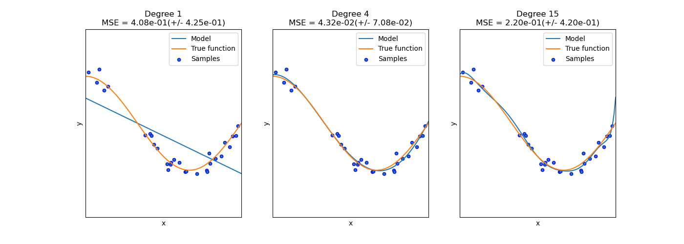
Polynominal Features

Add Feature Engineering with Polynominal Features. Guess the right value for degree parameter.

### Solution
from universe import *

import warnings
warnings.filterwarnings('ignore')  # To silence warnings

# Load Data
data = pd.read_csv('regression-lab-data-noisy.csv')
original_featureset = ['x0', 'x1', 'x2']
X = data[original_featureset]
y = data['y']
X_train, X_test, y_train, y_test = train_test_split(X, y, random_state=42)

# Fit Model
pipeline = Pipeline(steps=[
    ('onehot', OneHotEncoder(categorical_features=[2], sparse=False)),
    ('poly', PolynomialFeatures(degree=3, include_bias=False)),
    ('model', LinearRegression()),
])
pipeline.fit(X_train, y_train)

# Evaluate Model
train_score = pipeline.score(X_train, y_train)
test_score = pipeline.score(X_test, y_test)

# Print Results
print(f"INTERCEPT: {pipeline.named_steps['model'].intercept_}")
print(f"COEFFICIENTS: {pipeline.named_steps['model'].coef_}")
print(f"Train score: {train_score:.3f}")
print(f"Test score:  {test_score:.3f}")

INTERCEPT: 3.9222284624614225
COEFFICIENTS: [-4.28037041e-01  3.47535405e-01  8.05016356e-02 -2.04271240e+00
 -1.39694213e+00 -4.28037041e-01  1.35447209e-14  5.77315973e-15
 -1.71596933e+00 -9.21898626e-01  3.47535405e-01 -3.88578059e-15
  8.54668452e-01  1.15314113e-01  8.05016356e-02 -1.18141153e+00
 -5.90357612e-01  4.73940167e+00  1.25231340e+00  9.20134476e-01
 -4.28037041e-01  2.01948392e-28  0.00000000e+00 -1.71596933e+00
 -9.21898626e-01 -6.31088724e-30  0.00000000e+00  0.00000000e+00
  0.00000000e+00  0.00000000e+00  0.00000000e+00  0.00000000e+00
  2.97436479e+00  1.43788654e+00  4.44831435e-01  3.47535405e-01
  0.00000000e+00  8.54668452e-01  1.15314113e-01  0.00000000e+00
  0.00000000e+00  0.00000000e+00  6.17550505e-02 -2.10653204e+00
  1.70153048e-01  8.05016356e-02 -1.18141153e+00 -5.90357612e-01
  1.70328183e+00  1.92095889e+00  3.05149993e-01 -2.69542937e+00
 -4.60414672e+00 -1.00305071e-01 -5.73422478e-02]
Train score: 0.997
Test score:  0.963

Grid Search

Put the pipeline in a GridSearchCV and find optimal value for degree parameter in an automated way.

### Solution
from universe import *

import warnings
warnings.filterwarnings('ignore')  # To silence warnings

# Load Data
data = pd.read_csv('regression-lab-data-noisy.csv')
original_featureset = ['x0', 'x1', 'x2']
X = data[original_featureset]
y = data['y']
X_train, X_test, y_train, y_test = train_test_split(X, y, random_state=42)

# Fit Model
pipeline = Pipeline(steps=[
    ('onehot', OneHotEncoder(categorical_features=[2], sparse=False)),
    ('poly', PolynomialFeatures(include_bias=False)),
    ('model', LinearRegression()),
])
param_grid = {
    'poly__degree': [1, 2, 3],    
}                       
gs = GridSearchCV(
    pipeline,
    param_grid,
    cv=KFold(n_splits=5, random_state=42),
    iid=False,
    return_train_score=True,
)
gs.fit(X_train, y_train)

# Evaluate Model
test_score = gs.best_score_
final_score = gs.score(X_test, y_test)

# Print Results
print(f"INTERCEPT: {gs.best_estimator_.named_steps['model'].intercept_}")
print(f"COEFFICIENTS: {gs.best_estimator_.named_steps['model'].coef_}")
print(f"BEST PARAMS: {gs.best_params_}")
print(f"Test score: {test_score:.3f}")
print(f"Final evaluation score:  {final_score:.3f}")

INTERCEPT: 3.0458896606575863
COEFFICIENTS: [-1.00081669e+00  1.15488311e+00 -1.54066420e-01  1.03752181e+00
 -9.38017244e-01 -1.00081669e+00 -6.55935208e-16 -1.24991272e-16
  4.75744774e-01 -4.79473997e-01  1.15488311e+00  0.00000000e+00
  3.53422700e-01 -7.55868165e-01 -1.54066420e-01  2.08354336e-01
  2.97324918e-01 -4.00756753e-01 -3.49322903e+00  1.12969761e+00]
BEST PARAMS: {'poly__degree': 2}
Test score: 0.886
Final evaluation score:  0.954

Model Persistence

Saving

import pickle
stream = open('model.model', 'wb')
pickle.dump(gs.best_estimator_, stream)

Loading

import pickle
stream = open('model.model', 'rb')
pipeline = pickle.load(stream)

pipeline.predict(X_test)

array([0.06480651, 4.69147218, 1.98929037, 0.35971522, 4.62590384,
       5.55167464, 0.12810021, 1.16455893, 2.49774765])

Feature Engineering & Selection

from universe import *

Python version: 3.6.4
Universe has been successfully imported.

%matplotlib inline

Pipelines

Idea of Pipelines

PipelineFlow

Usage

### Hidden Cell -- just to make the usage working
X_train, y_train = np.array([[1]]), np.array([1])

pipeline = Pipeline(steps=[
    # Any number of transformers
    # ('poly', PolynomialFeatures()),  # example transformer
    # and then a model at the end of the pipeline 
    ('model', LinearRegression()),
])
pipeline.fit(X_train, y_train)
train_score = pipeline.score(X_train, y_train)
test_score = pipeline.score(X_test, y_test)
prediction = pipeline.predict(X_train)
coefs = pipeline.named_steps['model'].coef_
intercept = pipeline.named_steps['model'].intercept_

Exercise

from universe import *

# Dataset
dataset = pd.DataFrame({
    'group': [0,   0,   0,   1,   1,   1,   2,    2,    2],
    'x':     [10,  20,  30,  10,  20,  30,  10,   20,   30],
    'y':     [420, 440, 460, 120, 140, 160, 1020, 1040, 1060]
})
# y = 2*x + (300, 100 or 1000 depending on the group)

# Split dataset
X = dataset[['group', 'x']]
y = dataset['y']
X_train, y_train = X, y  # Use all data for training => no test set

### Exercise:
# 1) Build and Train Pipeline (use LinearRegression)
# 2) Make Prediction
# 3) Evaluate Model
# 4) Print Results

# Hints:
# dataset['new_column'] = ...  # Creates a new column

# ous model is predict = coef[0] * group + coef[1] * x + intercept

COEFFICIENTS: [300.   2.]
INTERCEPT: 200
Train score: 0.430

	group	x	y	predict
0	0	10	420	220.0
1	0	20	440	240.0
2	0	30	460	260.0
3	1	10	120	520.0
4	1	20	140	540.0
5	1	30	160	560.0
6	2	10	1020	820.0
7	2	20	1040	840.0
8	2	30	1060	860.0

One Hot Encoding

Usage

features = [0]  # indexes of categorical features
features = [True, False]  # or a mask
pipeline = Pipeline(steps=[
    ('onehot', OneHotEncoder(categorical_features=features, sparse=False)),
    ('model', LinearRegression()),
])

Exercise

Add one hot encoding to the previous exercise.

# Hint
import warnings
warnings.filterwarnings('ignore')  # To silence warnings

# predict_onehot = coef[group] + coef[3] * x + intercept

### Solution
pipeline = Pipeline(steps=[
    ('onehot', OneHotEncoder(
        categorical_features=[True, False], sparse=False)),
    ('model', LinearRegression()),
])
pipeline.fit(X_train, y_train)

# Predict
dataset['predict_onehot'] = pipeline.predict(X_train)

# Evaluate Model
train_score = pipeline.score(X_train, y_train)

# Print Results
coefs = pipeline.named_steps['model'].coef_
intercept = pipeline.named_steps['model'].intercept_
print(f"COEFFICIENTS: {pipeline.named_steps['model'].coef_}")
print(f"INTERCEPT: {pipeline.named_steps['model'].intercept_:.0f}")
print(f"Train score: {train_score:.3f}")
display(dataset)

COEFFICIENTS: [-100. -400.  500.    2.]
INTERCEPT: 500
Train score: 1.000

	group	x	y	predict	predict_onehot
0	0	10	420	220.0	420.0
1	0	20	440	240.0	440.0
2	0	30	460	260.0	460.0
3	1	10	120	520.0	120.0
4	1	20	140	540.0	140.0
5	1	30	160	560.0	160.0
6	2	10	1020	820.0	1020.0
7	2	20	1040	840.0	1040.0
8	2	30	1060	860.0	1060.0

Polynominal & Interaction Terms

Idea

X = np.array([[1, 20], [2, 30]])  # two features
poly = PolynomialFeatures(degree=3, include_bias=False)
poly.fit(X)
feature_names = poly.get_feature_names()
print("FEATURE NAMES:")
for feature in poly.get_feature_names():
    print("-", feature)

FEATURE NAMES:
- x0
- x1
- x0^2
- x0 x1
- x1^2
- x0^3
- x0^2 x1
- x0 x1^2
- x1^3

Example

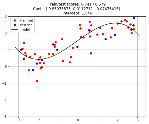
from universe import *

# Load and Split Data
X, y = mglearn.datasets.make_wave(n_samples=60)
y += 1.5
X_train, X_test, y_train, y_test = train_test_split(X, y, random_state=0)

# Define Model and Param Space
pipeline = Pipeline(steps=[
    ('poly', PolynomialFeatures(degree=3, include_bias=False)),
    ('model', LinearRegression()),
])

# Train Model with Grid Search and Cross Validation
pipeline.fit(X_train, y_train);

# Evaluate
train_score = pipeline.score(X_train, y_train)
test_score = pipeline.score(X_test, y_test)

# Plot Best Estimator
plt.figure(figsize=(8, 6))
plt.plot(X_train, y_train, 'o', color='r', label='train set')
plt.plot(X_test, y_test, 'o', color='b', label='test set')
xmin, xmax = plt.xlim()
xx = np.linspace(xmin, xmax).reshape(-1, 1)
yy = pipeline.predict(xx)
plt.plot(xx, yy, 'k', label='model')
plt.legend()
plt.title(f"Train/test scores: {train_score:.3f} / {test_score:.3f} \n"
f"Coefs: {pipeline.named_steps['model'].coef_} \n"
f"Intercept: {pipeline.named_steps['model'].intercept_:.3f}")
plt.ylim([-3, 3])
plt.grid()
plt.show()

Feature Selection

Strategies

1. Univariate Statistics: SelectKBest

Toy Dataset (Noised Breast Cancer)

from universe import *

# Load Dataset
cancer = load_breast_cancer()
X, y = cancer['data'], cancer['target']

# Add Noise Features to the Dataset
# get deterministic random numbers
rng = np.random.RandomState(42)
noise = rng.normal(size=(len(cancer.data), 50))
# add noise features to the data
# the first 30 features are from the dataset, the next 50 are noise
X_w_noise = np.hstack([X, noise])

# Split Dataset
X_train, X_test, y_train, y_test = train_test_split(
    X_w_noise, y, random_state=0, test_size=.5)

Compare Selectors

# Train and Evaluate Model without Feature Selection
model = LinearRegression()
model.fit(X_train, y_train)
train_score = model.score(X_train, y_train)
test_score = model.score(X_test, y_test)
print("                  train /  test  SELECTED INFORMATIVE FEATURES")
print(f"No selection    : {train_score:.3f} / {test_score:.3f}  " + "X"*30 + " (30 informative + 50 noisy)")

# Define Selectors
n_features = 20
selectors = [
    SelectKBest(k=n_features),
]

# Test Each Selector
for select in selectors:
    # Perform Feature Selection
    select.fit(X_train, y_train)

    # Transform Training set
    X_train_selected = select.transform(X_train)
    X_test_selected = select.transform(X_test)

    # Find Selected Features
    support = select.get_support()[:30].astype('int')
    chars = np.array([".", "X"])
    selected_features = "".join(chars[support])
    count = support.sum()

    # Train and Evaluate Model with Feature Selection
    model = LinearRegression()
    model.fit(X_train_selected, y_train)
    train_score = model.score(X_train_selected, y_train)
    test_score = model.score(X_test_selected, y_test)
    
    # Print Result
    print(f"{select.__class__.__name__:16}: {train_score:.3f} / {test_score:.3f}  {selected_features} ({count} informative + {n_features-count} noisy)")
    
print("")
print(f"X_train.shape:          {X_train.shape}")
print(f"X_train_selected.shape: {X_train_selected.shape}")

                  train /  test  SELECTED INFORMATIVE FEATURES
No selection    : 0.849 / 0.617  XXXXXXXXXXXXXXXXXXXXXXXXXXXXXX (30 informative + 50 noisy)
SelectKBest     : 0.783 / 0.730  XXXXXXXX..X.XX......XXXXXXXXX. (20 informative + 0 noisy)

X_train.shape:          (284, 80)
X_train_selected.shape: (284, 20)

Usage

pipeline = Pipeline(steps=[
    # Feature Engineering
    ('onehot', OneHotEncoder(categorical_features=[2], sparse=False)),
    ('poly', PolynomialFeatures(degree=2)),
    
    # Feature Selection
    ('select', SelectKBest(k=20)),
    
    # Model
    ('model', LinearRegression()),
])

Inception

from universe import *

Python version: 3.6.4
Universe has been successfully imported.

%matplotlib inline

Cross Validation

Why 80% / 20% for train/test?

• 99% / 1% => high variance

• 1% / 99% => high bias

• Cross Validation let us ensure that our evaluation has both low bias AND low variance.

Idea of Cross Validation

Cross Validation Strategies

k-Fold Cross Validation

from universe import *

X = np.array(["a", "b", "c", "d", "e", "f", "g", "h", "i"])
kf = KFold(n_splits=3)
print("Train set     test set")
for train_set, test_set in kf.split(X):
    print(f"{train_set} {test_set}")

Train set     test set
[3 4 5 6 7 8] [0 1 2]
[0 1 2 6 7 8] [3 4 5]
[0 1 2 3 4 5] [6 7 8]

Stratified k-Fold Cross Validation

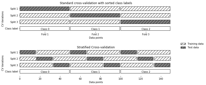
from universe import *
X = np.ones(10)
y = [0, 0, 0, 0, 1, 1, 1, 1, 1, 1]
skf = StratifiedKFold(n_splits=3)
print("Train set     test set")
for train_set, test_set in skf.split(X, y):
    print(f"{train_set} {test_set}")

Train set     test set
[2 3 6 7 8 9] [0 1 4 5]
[0 1 3 4 5 8 9] [2 6 7]
[0 1 2 4 5 6 7] [3 8 9]

Group K-Fold

from universe import *
X = range(10)
y = range(10)
# index:  0  1  2  3  4  5  6  7  8  9
groups = [1, 1, 1, 2, 2, 2, 3, 3, 2, 4]

print("K-FOLD")
kf = KFold(n_splits=3)
for train_set, test_set in kf.split(X, y):
    print(f"{train_set} {test_set}")

print("\nGROUP K-FOLD")
gkf = GroupKFold(n_splits=3)
for train_set, test_set in gkf.split(X, y, groups=groups):
    print(f"{train_set} {test_set}")

K-FOLD
[4 5 6 7 8 9] [0 1 2 3]
[0 1 2 3 7 8 9] [4 5 6]
[0 1 2 3 4 5 6] [7 8 9]

GROUP K-FOLD
[0 1 2 6 7 9] [3 4 5 8]
[3 4 5 6 7 8 9] [0 1 2]
[0 1 2 3 4 5 8] [6 7 9]

Time Series Split

from universe import *
X = y = range(12)
cv = TimeSeriesSplit(n_splits=3) 
for train_set, test_set in cv.split(X):
    print(f"{train_set} {test_set}")

[0 1 2] [3 4 5]
[0 1 2 3 4 5] [6 7 8]
[0 1 2 3 4 5 6 7 8] [ 9 10 11]

Grid Search

Idea of Grid Search

Usage

param_grid = {
    'model__n_neighbors': [1, 2, 3, 4],
    'poly__degree': [1, 2, 3],
}
pipeline = Pipeline(steps=[
    ('poly', PolynomialFeatures(include_bias=False)),
    ('model', KNeighborsClassifier()),
])
gs = GridSearchCV(
    pipeline, 
    param_grid, 
    cv=StratifiedKFold(n_splits=5, random_state=42),
    return_train_score=True,
    iid=False,
)
gs.fit(X_train, y_train);

Grid Search Outputs

print(f"BEST PARAMS: {gs.best_params_}")
print(f"VALIDATION SCORE: {gs.best_score_}")

n_neighbors = gs.best_params_['model__n_neighbors']
print(f"n_neighbors = {n_neighbors}")

n = gs.best_estimator_.named_steps['poly'].n_output_features_
print(f"OUTPUT FEATURES: {n}")

print(gs.best_estimator_.score(X_train, y_train) == gs.score(X_train, y_train))

BEST PARAMS: {'model__n_neighbors': 4, 'poly__degree': 1}
VALIDATION SCORE: 0.5905138339920949
n_neighbors = 4
OUTPUT FEATURES: 4
True

GridSearch.cvresults

display(pd.DataFrame(gs.cv_results_)[:3].T)

	0	1	2
mean_fit_time	0.00106659	0.00074439	0.00130987
mean_score_time	0.00146742	0.000961018	0.0012074
mean_test_score	0.563636	0.564032	0.518182
mean_train_score	1	1	1
param_model__n_neighbors	1	1	1
param_poly__degree	1	2	3
params	{'model__n_neighbors': 1, 'poly__degree': 1}	{'model__n_neighbors': 1, 'poly__degree': 2}	{'model__n_neighbors': 1, 'poly__degree': 3}
rank_test_score	5	4	11
split0_test_score	0.521739	0.478261	0.521739
split0_train_score	1	1	1
split1_test_score	0.478261	0.478261	0.478261
split1_train_score	1	1	1
split2_test_score	0.545455	0.5	0.363636
split2_train_score	1	1	1
split3_test_score	0.681818	0.727273	0.681818
split3_train_score	1	1	1
split4_test_score	0.590909	0.636364	0.545455
split4_train_score	1	1	1
std_fit_time	0.000432371	0.000154152	0.000797581
std_score_time	0.00109282	0.000235273	0.000197652
std_test_score	0.0694056	0.10069	0.102967
std_train_score	0	0	0

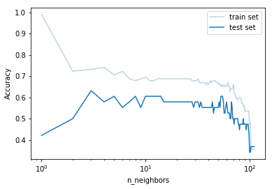
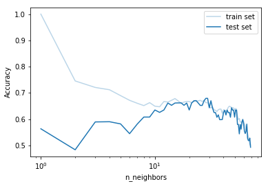
Grid Search Example

from universe import *

# Load and Split Data
iris = load_iris()
X, y = iris['data'], iris['target']
np.random.seed(0)
y[::2] = np.random.randint(0, 3, size=(y.size//2))  # add some noise
# train set is split into train and holdout sets during cross validation
X_train, X_test, y_train, y_test = train_test_split(
    X, y, random_state=0, stratify=y)

# Define Model and Param Space
param_grid = {
    'model__n_neighbors': np.arange(1, 70),
}
pipeline = Pipeline(steps=[
    ('model', KNeighborsClassifier())
])
gs = GridSearchCV(
    pipeline, 
    param_grid, 
    cv=StratifiedKFold(n_splits=5, random_state=42),
    return_train_score=True,
    iid=False,
)
gs.fit(X_train, y_train)

# Evaluate Model
final_score = gs.score(X_test, y_test)

# Summarize
print(f"Best params: {gs.best_params_}")
print(f"Test score: {gs.best_score_:.3f}")
print(f"Final score:       {final_score:.8f}")

# Prepare data for the plot
k = gs.cv_results_['param_model__n_neighbors']
train_scores = gs.cv_results_['mean_train_score']
test_scores = gs.cv_results_['mean_test_score']

# Plot
plt.plot(k, train_scores, 'C0', alpha=0.3, label="train set")
plt.plot(k, test_scores, 'C0', label="test set")
plt.ylabel("Accuracy")
plt.xlabel("n_neighbors")
plt.xscale('log')
plt.legend()
plt.show()

Best params: {'model__n_neighbors': 28}
Test score: 0.679
Final score:       0.60526316

Models

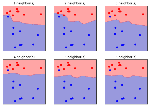
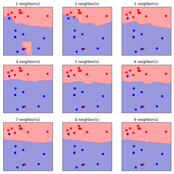
K-Nearest Neighbors

Scikit-learn Documentation on K-Nearest Neighbors Algorithm

k Parameter

from universe import *

# Load Data
X, y = mglearn.datasets.make_forge()
y[7] = 1
print(f"X[:5] = {X[:5]}")
print(f"y = {y}")

# Train/Test Set Split
forge_X_train, forge_X_test, forge_y_train, forge_y_test = \
    train_test_split(X, y, random_state=0)

# Train Models and Plot Figures
plt.figure(figsize=(10, 10))
for k in range(1, 10):
    plt.subplot(3, 3, k)
    
    # Train Model
    clf = KNeighborsClassifier(n_neighbors=k)
    clf.fit(forge_X_train, forge_y_train)

    # Plot Figure
    cmap = mpl.colors.ListedColormap(['b', 'r'])
    mglearn.plots.plot_2d_separator(clf, forge_X_train, fill=True, eps=0.5, alpha=.4)
    plt.scatter(forge_X_train[:, 0], forge_X_train[:, 1], c=forge_y_train, 
                cmap=cmap, s=40, lw=1)
    plt.title(f"{k} neighbor(s)")
plt.show()

X[:5] = [[ 9.96346605  4.59676542]
 [11.0329545  -0.16816717]
 [11.54155807  5.21116083]
 [ 8.69289001  1.54322016]
 [ 8.1062269   4.28695977]]
y = [1 0 1 0 0 1 1 1 1 1 1 1 0 0 1 1 1 0 0 1 0 0 0 0 1 0]

kNN for Regression

Linear & Logistic Regression

Linear Regression and Logistic Regression (which indeed is a Classification problem) were introduced in previous modules.

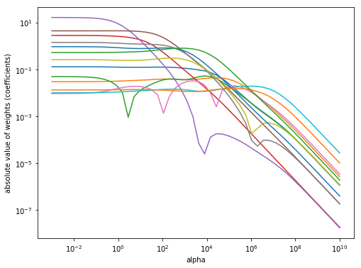
Ridge Regularization

Cost function

Cost function ($k$ features, $n$ samples):

$$ \underset{w_1,\dots,w_k,b}{min\,} \frac{1}{2n} \sum\limits_{i}^{n} (y_\textit{prediction} - y_\textit{ground truth})^2 + \alpha (w_1^2 + \dots + w_k^2 + b^2) $$

Regularization and Parameters

from universe import *

# Load and Split Data
dataset = load_boston()
X, y = dataset['data'], dataset['target']
feature_names = dataset['feature_names']
X_train, X_test, y_train, y_test = train_test_split(X, y, random_state=42)

# Train Model and Compute Results
def compute_coefs(alpha):
    model = Ridge(alpha=alpha)
    model.fit(X_train, y_train)
    return model.coef_
compute_coefs = np.vectorize(compute_coefs, signature='()->(n)')
    
alpha = np.logspace(-3, 10)
coefs = compute_coefs(alpha)

# Plot Figure
plt.figure(figsize=(8, 6))
plt.plot(alpha, np.abs(coefs))
plt.xscale('log')
plt.xlabel('alpha')
plt.ylabel('absolute value of weights (coefficients)')
plt.yscale('log')
plt.show()

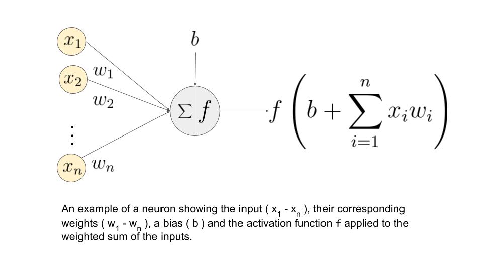
Neural Networks

Neuron

Neural Network

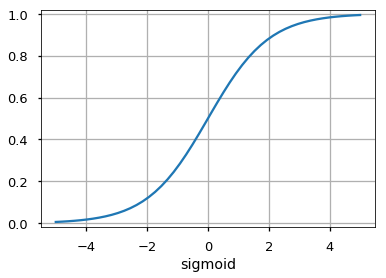
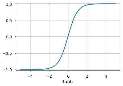
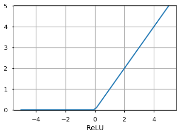
Activation Functions

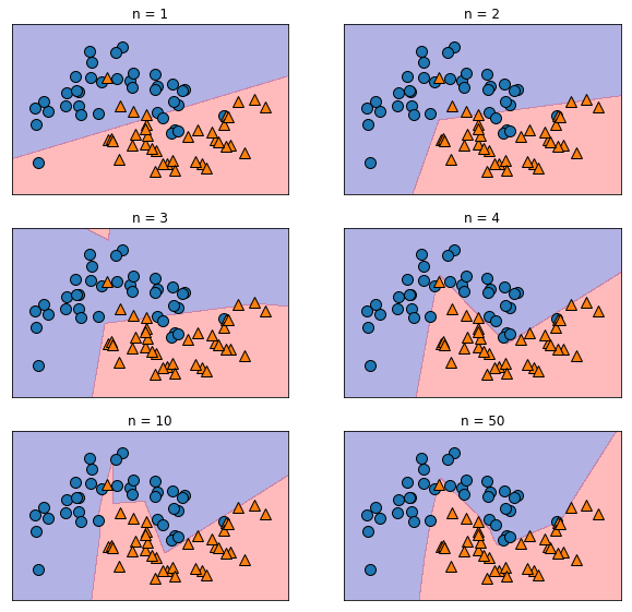
Number of Neurons

# Toy Dataset
X, y = make_moons(n_samples=100, noise=0.25, random_state=3)

X_train, X_test, y_train, y_test = train_test_split(
    X, y, stratify=y, random_state=42)

# 
plt.figure(figsize=(10,20))
i = 1
for n in [1, 2, 3, 4, 10, 50]:
    mlp = MLPClassifier(solver='lbfgs', activation='relu', 
                        random_state=0, hidden_layer_sizes=[n])
    mlp.fit(X_train, y_train)

    plt.subplot(6, 2, i)
    plt.title(f"n = {n}")
    mglearn.plots.plot_2d_separator(mlp, X_train, fill=True, alpha=.3)
    mglearn.discrete_scatter(X_train[:, 0], X_train[:, 1], y_train)
    i += 1
plt.show()

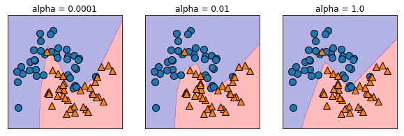
Regularization

plt.figure(figsize=(10, 3))
for i, alpha in enumerate([0.0001, 0.01, 1.0]):
    mlp = MLPClassifier(solver='lbfgs', random_state=0,
                        hidden_layer_sizes=[20, 20], alpha=alpha)
    mlp.fit(X_train, y_train)
    plt.subplot(1, 3, i+1)
    mglearn.plots.plot_2d_separator(mlp, X_train, fill=True, alpha=.3)
    mglearn.discrete_scatter(X_train[:, 0], X_train[:, 1], y_train)
    plt.title(f"alpha = {alpha}")
plt.show()

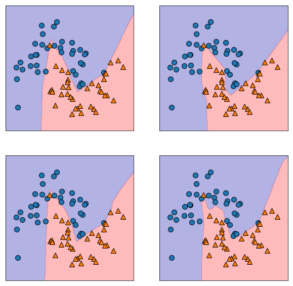
Randomness

plt.figure(figsize=(10, 10))
for i in range(4):
    plt.subplot(2, 2, i+1)
    mlp = MLPClassifier(solver='lbfgs', random_state=i,
                        hidden_layer_sizes=[20, 20])
    mlp.fit(X_train, y_train)
    mglearn.plots.plot_2d_separator(mlp, X_train, fill=True, alpha=.3)
    mglearn.discrete_scatter(X_train[:, 0], X_train[:, 1], y_train)
plt.show()

Decision Trees

Decision Tree Building - Divide and Conquer

Controlling Tree Complexity

from universe import *
cancer = load_breast_cancer()
X_train, X_test, y_train, y_test = train_test_split(
    cancer.data, cancer.target, stratify=cancer.target, random_state=42)

tree = DecisionTreeClassifier(random_state=0)
tree.fit(X_train, y_train)
training_score = tree.score(X_train, y_train)
test_score = tree.score(X_test, y_test)
print("WITHOUT PRE-PRUNNING")
print(f"Accuracy on training set: {training_score:.3f}")
print(f"Accuracy on test set: {test_score:.3f}")

tree = DecisionTreeClassifier(max_depth=2, random_state=0)
tree.fit(X_train, y_train)
training_score = tree.score(X_train, y_train)
test_score = tree.score(X_test, y_test)
print("")
print("WITH PRE-PRUNNING")
print(f"Accuracy on training set: {training_score:.3f}")
print(f"Accuracy on test set: {test_score:.3f}")

WITHOUT PRE-PRUNNING
Accuracy on training set: 1.000
Accuracy on test set: 0.937

WITH PRE-PRUNNING
Accuracy on training set: 0.958
Accuracy on test set: 0.909

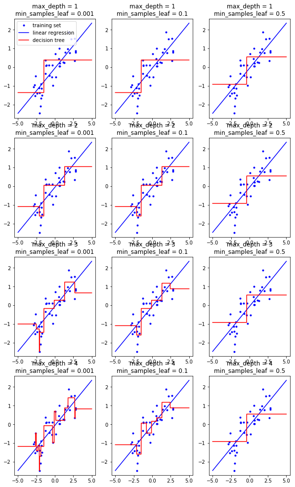
Decision Tree for Regression

from universe import *

X, y = mglearn.datasets.make_wave(n_samples=40)

### Exercise: Plot the Figure
# Hint:
'''
i = 1
for max_depth in [1, 2, 3, 4]:
    for min_samples_leaf in [0.001, 0.1, 0.5]:
        plt.subplot(4, 3, i)
        tree = DecisionTreeRegressor(
            max_depth=max_depth, 
            min_samples_leaf=min_samples_leaf)
        ...
        i += 1
plt.show()
''';

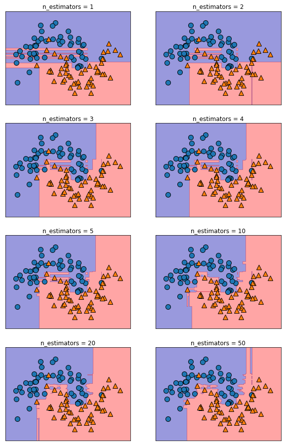
Random Forests

Random Forests

from universe import *

X, y = make_moons(n_samples=100, noise=0.25, random_state=3)

i = 1
plt.figure(figsize=(10, 16))
for n_estimators in [1, 2, 3, 4, 5, 10, 20, 50]:
    forest = RandomForestClassifier(n_estimators=n_estimators, random_state=2)
    forest.fit(X, y);

    plt.subplot(4, 2, i)
    plt.title(f"n_estimators = {n_estimators}")
    mglearn.plots.plot_2d_separator(forest, X, fill=True,
                                    alpha=.4)
    mglearn.discrete_scatter(X[:, 0], X[:, 1], y)
    i += 1
plt.show()

forest = RandomForestClassifier(max_leaf_nodes=4, n_estimators=3, random_state=2)
forest.fit(X, y)
tree1, tree2, tree3 = forest.estimators_

def display_tree(tree, feature_names):
    dot_data = export_graphviz(
        tree, out_file=None, 
        feature_names=feature_names, label='root', 
        filled=True, impurity=False)
    display(graphviz.Source(dot_data))

display_tree(tree1, feature_names=['X[0]', 'X[1]'])

display_tree(tree2, feature_names=['X[0]', 'X[1]'])

display_tree(tree3, feature_names=['X[0]', 'X[1]'])

X_test = np.array([[2, 3]])
print(tree1.predict(X_test))
print(tree2.predict(X_test))
print(tree3.predict(X_test))
print(forest.predict(X_test))

[1.]
[0.]
[0.]
[0]

Classification

from universe import *

Python version: 3.6.4
Universe has been successfully imported.

%matplotlib inline

Logistic Regression

Scikit-learn Documentation on Logistic Regression

Odds Ratio

$$ Odds=\frac{p}{1-p}$$

$$ p=\frac{Odds}{1+Odds} $$

Assume that probability is in $(0, 1)$ range, excluding 0 and 1.

=> Odds Ratio is in $(0,+\infty)$ range.

=> Logarithm of Odds Ratio is in $(-\infty, +\infty)$ range.

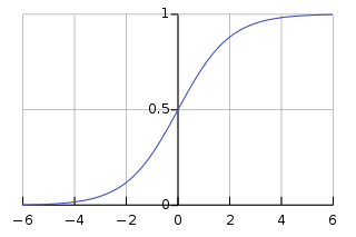
Logit function is defined as logarithm of odds ratio. We model it with a linear combination:

$$ \operatorname{logit}(p)=\ln\left(\frac{p}{1-p}\right) = w_1 x_{1} + \cdots + w_k x_{k} + b$$

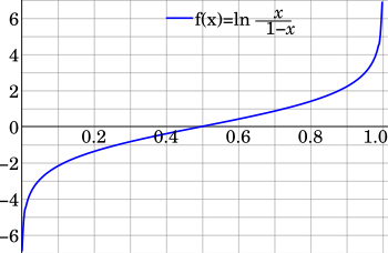
We can compute the probability back from its logit. This is called Logistic Function:

$$ p =\frac{e^{\operatorname{logit}(p)}}{1+e^{\operatorname{logit}(p)}} =\frac{1}{1+e^{-\operatorname{logit}(p)}} =\frac{1}{1+e^{-(w_1 x_{1} + \cdots + w_k x_{k} + c)}} $$

Cost Function

L2 Regularization:

$$\underset{w, c}{min\,} \frac{1}{2}\left(w_1^2+\cdots+w_k^2\right) + C \sum_{i=1}^n \ln\left(1 + e^{- y_i (w_1 x_{i,1} + \cdots + w_k x_{i,k} + c)} \right)$$

Binary Classification

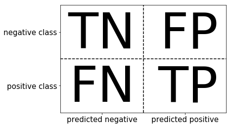
Confusion Matrix

Beyond Accuracy

Consider a test that can be positive or negative. This test tells you if somebody is drug user or not.

Accuracy -- how often we get correct result (doesn't matter if it's negative or positive)?

$$Accuracy = \frac{TP + TN}{TP + TN + FP + FN}$$

Precision, positive predictive value (PPV) -- when test is positive, how likely it's that one is drug user?

$$Precision = \frac{TP}{TP + FP}$$

Recall, sensitivity, hit rate, true positive rate (TPR) -- when one is drug user, how likely it is that the test will detect it, that is it's positive? $$Recall = \frac{TP}{TP + FN}$$

$F_1$-score -- a metric combining both Precision and Recall.

$$F = 2 \cdot \frac{precision \cdot recall}{precision + recall} = \frac{2}{\frac{1}{precision}+\frac{1}{recall}}$$

Polish names:

• Accuracy = dokładność
• Precision = precyzja
• Recall = czułość

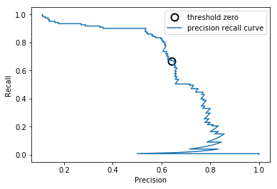
Precision-Recall Curve

from universe import *

# Load Data and Split It
X, y = mglearn_make_blobs(n_samples=(4000, 500), centers=2, cluster_std=[7.0, 2],
                          random_state=22)
X_train, X_test, y_train, y_test = train_test_split(X, y, random_state=0)

# Build And Train Model
svc = SVC(gamma=.05).fit(X_train, y_train)

# Compute Precision-Recall Curve
precision, recall, thresholds = precision_recall_curve(
    y_test, svc.decision_function(X_test))

# Find threshold closest to zero
close_zero = np.argmin(np.abs(thresholds))

# Plot Precision-Recall Curve
plt.plot(precision[close_zero], recall[close_zero], 'o', markersize=10,
         label="threshold zero", fillstyle="none", c='k', mew=2)
plt.plot(precision, recall, label="precision recall curve")
plt.xlabel("Precision")
plt.ylabel("Recall")
plt.legend()
plt.show()

Usage with Grid Search

grid = GridSearchCV(
    pipeline,
    param_grid, 
    cv=KFold(n_split=5),
    refit='f1_score',
    return_train_score=True,
    iid=False,
)